Choosing a corrector: AutoCorrector and BatchCorrectionBenchmark#
MaldiBatchKit ships several correctors with overlapping use cases. Two v0.2 classes turn the which one should I use? question into an automated, scikit-learn-shaped workflow:
`AutoCorrector<https://maldibatchkit.readthedocs.io/en/latest/api/corrections.html#maldibatchkit.AutoCorrector>`__ exposes the correction method itself as a settable hyperparameter, so a singleGridSearchCVcan sweep across corrector families and let the downstream classifier metric (typically AUROC) pick the winner.`BatchCorrectionBenchmark<https://maldibatchkit.readthedocs.io/en/latest/api/diagnostics.html#maldibatchkit.diagnostics.BatchCorrectionBenchmark>`__ runs a fixed set of batch-mixing diagnostics across multiple correctors under a single protocol, with bootstrap confidence intervals.
The two tools answer different questions; pick the one that matches the decision you actually need to make.
Uses the MALDI-Kleb-AI dataset (Rocchi et al. 2026, Zenodo DOI 10.5281/zenodo.17405072).
1. Load the dataset#
[1]:
import sys, pathlib
sys.path.insert(0, str(pathlib.Path.cwd().parent))
from notebooks._demo import load_maldi_kleb_ai

demo = load_maldi_kleb_ai(antibiotic='Amikacin')
X = demo.X
batch = demo.batch          # Rome / Milan / Catania
species = demo.species      # K. pneumoniae / K. variicola / ...
quality = demo.meta['SNR']  # signal-to-noise ratio per spectrum
y = (demo.meta['Amikacin'] == 'R').astype(int)

print(f'X:       {X.shape}')
print(f'batches: {sorted(batch.unique())}')
print(f'species: {sorted(species.unique())}')
print(f'prevalence of resistance: {y.mean():.2%}')
X:       (741, 6000)
batches: ['Catania', 'Milan', 'Rome']
species: ['Klebsiella aerogenes', 'Klebsiella oxytoca', 'Klebsiella pneumoniae', 'Klebsiella variicola']
prevalence of resistance: 49.80%
2. AutoCorrector - swap the method as a hyperparameter#
AutoCorrector is a thin BaseBatchCorrector whose method argument selects an inner corrector at fit time. It accepts string aliases ('combat-fortin', 'harmony', 'qw-combat', 'noop', …) or a BaseBatchCorrector subclass. Covariates are routed to whatever the inner method actually understands:
discrete_covariates→ ComBat’sdiscrete_covariates, Harmony’scovariates, Limma’sdesign,continuous_covariates→ ComBat only,quality→QualityWeightedComBat.quality,species→SpeciesAwareComBat.species.
Anything the inner does not accept is dropped silently (sklearn convention), so the same param_grid can target multiple methods.
[2]:
import warnings
from maldibatchkit import AutoCorrector

ac = AutoCorrector(
    batch=batch,
    method='combat-fortin',
    discrete_covariates=species,
    quality=quality,          # ignored by combat-fortin
)
ac.fit(X)
print('inner class:', type(ac.inner_).__name__)

# Switch to QualityWeightedComBat. `quality=` is now consumed;
# `discrete_covariates=` is the one being dropped. AutoCorrector
# emits a UserWarning for every dropped kwarg; we capture it here
# explicitly so the demo output stays tidy.
ac.set_params(method='qw-combat')
with warnings.catch_warnings(record=True) as wlog:
    warnings.simplefilter('always')
    ac.fit(X)
print('inner class:', type(ac.inner_).__name__)
print('dropped kwargs warnings:')
for w in wlog:
    print(' -', w.message)
print('gamma_star_ shape (mirrored via __getattr__):', ac.gamma_star_.shape)
inner class: ComBat
inner class: QualityWeightedComBat
dropped kwargs warnings:
 - method='qw-combat' does not accept discrete covariates; ignoring `discrete_covariates`.
gamma_star_ shape (mirrored via __getattr__): (3, 6000)
2.1. Cross-validated per-batch AUROC#
Overall AUROC can hide site-specific failures: a model can score 0.80 overall while being near-random on the smallest site. If a corrector truly removes batch effect useful for the task, the per-batch AUROC should tighten around the overall value rather than diverge across the three sites.
We run a 5-fold CV stratified jointly by batch × y, so every fold sees the same per-site resistance prevalence. For each method we score AUROC per batch in the held-out fold, then aggregate across folds.
[3]:
import warnings
import numpy as np
import pandas as pd
from sklearn.base import clone
from sklearn.linear_model import LogisticRegression
from sklearn.metrics import roc_auc_score
from sklearn.model_selection import StratifiedKFold
from sklearn.pipeline import Pipeline
from sklearn.preprocessing import StandardScaler

methods = ['noop', 'median', 'combat-fortin', 'harmony']

base_pipe = Pipeline([
    ('correct', AutoCorrector(batch=batch,
                              discrete_covariates=species,
                              method_kwargs={'verbose': False,
                                             'random_state': 0,
                                             'n_components': 30})),
    ('scaler', StandardScaler()),
    ('clf', LogisticRegression(max_iter=1000, C=0.1, n_jobs=1)),
])

# Combine batch and outcome into a single stratification label so each
# fold sees the same per-site resistance prevalence.
strat = batch.astype(str) + '|' + y.astype(str)
cv_strat = StratifiedKFold(n_splits=5, shuffle=True, random_state=0)

records = []
with warnings.catch_warnings():
    warnings.simplefilter('ignore')
    for fold, (tr, te) in enumerate(cv_strat.split(X, strat)):
        X_tr, X_te = X.iloc[tr], X.iloc[te]
        y_tr, y_te = y.iloc[tr], y.iloc[te]
        b_te = batch.iloc[te].to_numpy()
        for m in methods:
            pipe = clone(base_pipe)
            pipe.set_params(correct__method=m)
            pipe.fit(X_tr, y_tr)
            proba = pipe.predict_proba(X_te)[:, 1]
            # overall fold AUROC
            records.append({
                'method': m, 'batch': '(overall)', 'fold': fold,
                'n': len(y_te), 'prev': float(y_te.mean()),
                'auc': roc_auc_score(y_te, proba),
            })
            # per-batch AUROC
            for lvl in sorted(batch.unique()):
                mask = b_te == lvl
                y_lvl = y_te.iloc[mask]
                if mask.sum() < 5 or y_lvl.nunique() < 2:
                    auc = np.nan
                else:
                    auc = roc_auc_score(y_lvl, proba[mask])
                records.append({
                    'method': m, 'batch': lvl, 'fold': fold,
                    'n': int(mask.sum()),
                    'prev': float(y_lvl.mean()) if mask.any() else np.nan,
                    'auc': auc,
                })

per_batch = pd.DataFrame(records)
summary = (per_batch
           .groupby(['method', 'batch'])['auc']
           .agg(['mean', 'std'])
           .round(4)
           .reset_index())
auc_pivot = summary.pivot(index='method', columns='batch', values='mean')
auc_pivot = auc_pivot.reindex(methods)        # keep our method order
auc_pivot = auc_pivot[sorted(batch.unique()) + ['(overall)']]
auc_pivot.round(4)
[3]:
| batch | Catania | Milan | Rome | (overall) |
|---|---|---|---|---|
| method | ||||
| noop | 0.8980 | 0.8258 | 0.6991 | 0.8147 |
| median | 0.8825 | 0.7902 | 0.7070 | 0.8129 |
| combat-fortin | 0.7995 | 0.8299 | 0.7021 | 0.7456 |
| harmony | 0.7588 | 0.6853 | 0.6439 | 0.7768 |
[4]:
# Spread across sites: range and standard deviation of the three
# per-batch AUROCs (smaller = better aligned).
per_site = auc_pivot.drop(columns='(overall)')
alignment = pd.DataFrame({
    'mean_per_site': per_site.mean(axis=1).round(4),
    'range':         (per_site.max(axis=1) - per_site.min(axis=1)).round(4),
    'std':           per_site.std(axis=1).round(4),
    'overall':       auc_pivot['(overall)'].round(4),
})
alignment.sort_values('range')
[4]:
| mean_per_site | range | std | overall | |
|---|---|---|---|---|
| method | ||||
| harmony | 0.6960 | 0.1149 | 0.0582 | 0.7768 |
| combat-fortin | 0.7772 | 0.1278 | 0.0668 | 0.7456 |
| median | 0.7932 | 0.1755 | 0.0878 | 0.8129 |
| noop | 0.8076 | 0.1989 | 0.1007 | 0.8147 |
2.2. Picking the winner with make_batch_scorer#
The manual CV table above is informative but tedious. maldibatchkit.metrics ships make_batch_scorer, which packages a per-batch metric with a chosen across-batch aggregation as a sklearn scorer. Drop it into GridSearchCV(scoring=...) and the right corrector falls out automatically.
The weights= argument controls how the per-batch scalars are aggregated:
weights='size'weights each site by its sample count. For additive metrics whose definition iscorrect / total(accuracy, error rate), this exactly recovers the standard pooled value. For metrics with a class-conditional denominator (sensitivity, specificity), recovering the pooled value needs class-conditional weights, not size weights. For non-linear metrics (F1, precision, MCC, balanced accuracy), no per-batch weighting recovers pooled exactly. For AUROC and average precision, pooled values count cross-batch positive-vs-negative pairs that any per-batch reducer cannot see by construction - they are gone, not approximated. In every non-additive case the dominant site still dominates the score in the same direction.weights='uniform'gives each site equal weight - one vote per site - so a corrector that bombs on a small site is properly penalised. The right choice when the goal is a classifier that generalises across sites.weights='balanced'weights each site inversely by its sample count (w_i ∝ 1 / n_i), mirroring sklearn’sclass_weight='balanced'formula at the per-batch level. The smallest site gets the loudest voice. Use this when minority sites are the hardest distributions to learn and the corrector must not crush them.a
{batch_label: weight}dict lets you encode any custom policy.
Switching weighting modes typically picks different winners, which is exactly the trade-off we want the user to make explicit.
[5]:
from maldibatchkit.metrics import make_batch_scorer
from sklearn.model_selection import GridSearchCV

# Materialise the CV folds once so both grid searches see the same
# train / test splits (cv_strat.split returns a one-shot generator).
folds = list(cv_strat.split(X, strat))

weight_modes = ('size', 'uniform', 'balanced')
picks = {}
for weights_mode in weight_modes:
    scorer = make_batch_scorer(batch, metric='roc_auc', weights=weights_mode)
    grid = GridSearchCV(
        base_pipe,
        param_grid={'correct__method': methods},
        scoring=scorer,
        cv=folds,
        n_jobs=1,
    )
    with warnings.catch_warnings():
        warnings.simplefilter('ignore')
        grid.fit(X, y)
    picks[weights_mode] = (
        pd.DataFrame(grid.cv_results_)
          [['param_correct__method', 'mean_test_score', 'std_test_score']]
          .rename(columns={
              'param_correct__method': 'method',
              'mean_test_score': f'mean_{weights_mode}',
              'std_test_score':  f'std_{weights_mode}',
          })
    )

comparison = picks['size']
for m in ('uniform', 'balanced'):
    comparison = comparison.merge(picks[m], on='method')
comparison = (comparison
              .sort_values('mean_uniform', ascending=False)
              .reset_index(drop=True)
              .round(4))
comparison
[5]:
| method | mean_size | std_size | mean_uniform | std_uniform | mean_balanced | std_balanced | |
|---|---|---|---|---|---|---|---|
| 0 | noop | 0.7541 | 0.0495 | 0.8076 | 0.0527 | 0.8550 | 0.0626 |
| 1 | median | 0.7484 | 0.0570 | 0.7932 | 0.0593 | 0.8363 | 0.0673 |
| 2 | combat-fortin | 0.7451 | 0.0232 | 0.7772 | 0.0275 | 0.7975 | 0.0723 |
| 3 | harmony | 0.6678 | 0.0184 | 0.6960 | 0.0458 | 0.7246 | 0.0640 |
[6]:
# Which corrector each weighting mode picks (best mean score).
winners = {
    mode: df.set_index('method')[f'mean_{mode}'].idxmax()
    for mode, df in picks.items()
}
winners
[6]:
{'size': 'noop', 'uniform': 'noop', 'balanced': 'noop'}
3. BatchCorrectionBenchmark - diagnostic comparison#
BatchCorrectionBenchmark is the diagnostic counterpart: configure once, then .fit(X, batch=..., species=...) to score every corrector against every metric. It is diagnostic-only by design - no downstream classifier is involved. The output is a tidy (method, metric, value, ci_lo, ci_hi, std, n, better) table ready for paper-figure comparisons.
Bootstrap confidence intervals are stratified by batch:
bootstrap_mode='resample_metric'(default, fast) - fit each corrector once, resample rows of the corrected matrix to give the CI.bootstrap_mode='refit'(slower) - resample rows ofXand refit per bootstrap iteration. The CI then also captures corrector stability.
[7]:
from maldibatchkit import (
    ComBat, Harmony, Limma, NoOpCorrector, QualityWeightedComBat, SpeciesAwareComBat,
)
from maldibatchkit.diagnostics import BatchCorrectionBenchmark

bench = BatchCorrectionBenchmark(
    correctors={
        'none':           NoOpCorrector(batch=batch),
        'limma':          Limma(batch=batch, design=pd.get_dummies(species).astype(float)),
        'combat-johnson': ComBat(batch=batch, method='johnson'),
        'combat-fortin':  ComBat(batch=batch, method='fortin',
                                 discrete_covariates=species),
        'species-combat': SpeciesAwareComBat(batch=batch, species=species),
        'qw-combat':      QualityWeightedComBat(batch=batch, quality=quality),
        'harmony':        Harmony(batch=batch, covariates=species,
                                  n_components=30, verbose=False,
                                  random_state=0),
    },
    metrics=(
        'silhouette_batch',
        'kbet',
        'lisi_normalized',
        'species_preservation',
    ),
    n_bootstrap=50,
    bootstrap_mode='resample_metric',
    random_state=0,
)
bench.fit(X, batch=batch, species=species)
bench.results_.round(4)
[7]:
| method | metric | value | ci_lo | ci_hi | std | n | better | |
|---|---|---|---|---|---|---|---|---|
| 0 | none | silhouette_batch | 0.1490 | 0.1408 | 0.1582 | 0.0054 | 51.0 | zero |
| 1 | none | kbet | 0.0212 | 0.0094 | 0.0364 | 0.0073 | 51.0 | higher |
| 2 | none | lisi_normalized | 0.4902 | 0.4842 | 0.4978 | 0.0039 | 51.0 | higher |
| 3 | none | species_preservation | 1.0000 | 1.0000 | 1.0000 | 0.0000 | 51.0 | higher |
| 4 | limma | silhouette_batch | 0.0279 | 0.0142 | 0.0435 | 0.0083 | 51.0 | zero |
| 5 | limma | kbet | 0.1032 | 0.0661 | 0.1248 | 0.0167 | 51.0 | higher |
| 6 | limma | lisi_normalized | 0.5146 | 0.5039 | 0.5280 | 0.0062 | 51.0 | higher |
| 7 | limma | species_preservation | 1.0000 | 1.0000 | 1.0000 | 0.0000 | 51.0 | higher |
| 8 | combat-johnson | silhouette_batch | -0.0095 | -0.0282 | 0.0051 | 0.0090 | 51.0 | zero |
| 9 | combat-johnson | kbet | 0.2338 | 0.1866 | 0.2871 | 0.0279 | 51.0 | higher |
| 10 | combat-johnson | lisi_normalized | 0.6447 | 0.6215 | 0.6660 | 0.0129 | 51.0 | higher |
| 11 | combat-johnson | species_preservation | 0.9156 | 0.8368 | 0.9773 | 0.0408 | 51.0 | higher |
| 12 | combat-fortin | silhouette_batch | -0.0094 | -0.0219 | 0.0018 | 0.0077 | 51.0 | zero |
| 13 | combat-fortin | kbet | 0.2289 | 0.1815 | 0.2848 | 0.0311 | 51.0 | higher |
| 14 | combat-fortin | lisi_normalized | 0.6272 | 0.6063 | 0.6472 | 0.0117 | 51.0 | higher |
| 15 | combat-fortin | species_preservation | 0.9826 | 0.9444 | 1.0000 | 0.0186 | 51.0 | higher |
| 16 | species-combat | silhouette_batch | -0.0121 | -0.0344 | 0.0032 | 0.0096 | 51.0 | zero |
| 17 | species-combat | kbet | 0.2328 | 0.1876 | 0.2881 | 0.0291 | 51.0 | higher |
| 18 | species-combat | lisi_normalized | 0.6283 | 0.6047 | 0.6519 | 0.0139 | 51.0 | higher |
| 19 | species-combat | species_preservation | 0.9777 | 0.9361 | 1.0000 | 0.0232 | 51.0 | higher |
| 20 | qw-combat | silhouette_batch | 0.0108 | -0.0003 | 0.0196 | 0.0053 | 51.0 | zero |
| 21 | qw-combat | kbet | 0.1818 | 0.1407 | 0.2196 | 0.0213 | 51.0 | higher |
| 22 | qw-combat | lisi_normalized | 0.6086 | 0.5886 | 0.6276 | 0.0117 | 51.0 | higher |
| 23 | qw-combat | species_preservation | 0.9218 | 0.8512 | 0.9892 | 0.0375 | 51.0 | higher |
| 24 | harmony | silhouette_batch | 0.0452 | 0.0336 | 0.0564 | 0.0065 | 51.0 | zero |
| 25 | harmony | kbet | 0.1289 | 0.0962 | 0.1680 | 0.0192 | 51.0 | higher |
| 26 | harmony | lisi_normalized | 0.6386 | 0.5964 | 0.6828 | 0.0221 | 51.0 | higher |
| 27 | harmony | species_preservation | 0.7245 | 0.6017 | 0.8224 | 0.0646 | 51.0 | higher |
Sort by any metric - .rank() follows the metric’s registered direction ('higher' → descending, 'lower' → ascending) by default. Here species_preservation ∈ [0, 1] where 1 means species are perfectly preserved after correction.
[8]:
bench.rank('species_preservation').round(4)
[8]:
| method | metric | value | ci_lo | ci_hi | std | n | better | |
|---|---|---|---|---|---|---|---|---|
| 0 | none | species_preservation | 1.0000 | 1.0000 | 1.0000 | 0.0000 | 51.0 | higher |
| 1 | limma | species_preservation | 1.0000 | 1.0000 | 1.0000 | 0.0000 | 51.0 | higher |
| 2 | combat-fortin | species_preservation | 0.9826 | 0.9444 | 1.0000 | 0.0186 | 51.0 | higher |
| 3 | species-combat | species_preservation | 0.9777 | 0.9361 | 1.0000 | 0.0232 | 51.0 | higher |
| 4 | qw-combat | species_preservation | 0.9218 | 0.8512 | 0.9892 | 0.0375 | 51.0 | higher |
| 5 | combat-johnson | species_preservation | 0.9156 | 0.8368 | 0.9773 | 0.0408 | 51.0 | higher |
| 6 | harmony | species_preservation | 0.7245 | 0.6017 | 0.8224 | 0.0646 | 51.0 | higher |
[9]:
bench.rank('silhouette_batch').round(4)
[9]:
| method | metric | value | ci_lo | ci_hi | std | n | better | |
|---|---|---|---|---|---|---|---|---|
| 0 | combat-fortin | silhouette_batch | -0.0094 | -0.0219 | 0.0018 | 0.0077 | 51.0 | zero |
| 1 | combat-johnson | silhouette_batch | -0.0095 | -0.0282 | 0.0051 | 0.0090 | 51.0 | zero |
| 2 | qw-combat | silhouette_batch | 0.0108 | -0.0003 | 0.0196 | 0.0053 | 51.0 | zero |
| 3 | species-combat | silhouette_batch | -0.0121 | -0.0344 | 0.0032 | 0.0096 | 51.0 | zero |
| 4 | limma | silhouette_batch | 0.0279 | 0.0142 | 0.0435 | 0.0083 | 51.0 | zero |
| 5 | harmony | silhouette_batch | 0.0452 | 0.0336 | 0.0564 | 0.0065 | 51.0 | zero |
| 6 | none | silhouette_batch | 0.1490 | 0.1408 | 0.1582 | 0.0054 | 51.0 | zero |
The raw observations are kept in results_long_ (one row per (method, metric, repeat, bootstrap)). The point estimate is marked bootstrap == -1; the resampled values are bootstrap >= 0. Use it to compute custom statistics or to drive a raincloud / strip plot.
[10]:
bench.results_long_.head()
[10]:
| method | metric | repeat | bootstrap | value | |
|---|---|---|---|---|---|
| 0 | none | silhouette_batch | 0 | -1 | 0.147457 |
| 1 | none | kbet | 0 | -1 | 0.020243 |
| 2 | none | lisi_normalized | 0 | -1 | 0.484701 |
| 3 | none | species_preservation | 0 | -1 | 1.000000 |
| 4 | none | silhouette_batch | 0 | 0 | 0.143741 |
[11]:
# Baseline metrics on the *uncorrected* X (a useful reference line in plots).
bench.baseline_.round(4)
[11]:
| method | metric | value | ci_lo | ci_hi | std | n | better | |
|---|---|---|---|---|---|---|---|---|
| 0 | __baseline__ | silhouette_batch | 0.1475 | NaN | NaN | NaN | 1 | zero |
| 1 | __baseline__ | kbet | 0.0202 | NaN | NaN | NaN | 1 | higher |
| 2 | __baseline__ | lisi_normalized | 0.4847 | NaN | NaN | NaN | 1 | higher |
| 3 | __baseline__ | species_preservation | 1.0000 | NaN | NaN | NaN | 1 | higher |
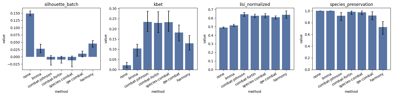
And the convenience .plot() helper, faceted by metric with the bootstrap CIs as error bars:
[12]:
import matplotlib.pyplot as plt  # noqa: F401
%matplotlib inline
bench.plot();
4. Which tool when?#
``AutoCorrector`` inside a stratified CV loop - when the question is does this correction make my AMR classifier better, on every site? The downstream classifier metric is the only honest arbiter of whether the correction step helps the task you actually care about. Do not read only the overall AUROC: stratify the held-out folds jointly by
batch × yand look at the per-batch table. A method that ‘improves’ the mean while still leaving a large gap between sites is buying alignment at the cost of overall performance - or buying overall performance by riding site-specific signal that won’t transfer.``BatchCorrectionBenchmark`` - when the question is which corrector mixes batches and preserves species best, independent of any classifier? (method-comparison tables, deciding whether a corrector is blurring biology). Cheap, downstream-agnostic, and reproducible via the stratified bootstrap CIs.
The two tools disagree on this cohort - and that disagreement is the lesson#
The diagnostic table ranks ComBat variants on top: they flatten the batch axis, the LISI normalised score climbs, species preservation stays near-perfect. The per-batch AUROC table puts noop and median on top: the uncorrected matrix produces the highest mean per-site AUROC, and the widest cross-site spread.
That gap between the two verdicts is not a bug in either tool. It is the classic multi-centre clinical-AMR trap: inter-site differences are partly the resistance signal itself - different patient populations, different antibiograms, different colonisation pressure. Aggressive batch correction is mathematically obliged to strip that signal because the corrector has no way to know which inter-site differences are ‘real’ biology and which are technical drift.
MaldiBatchKit cannot make that decision for you. What it does is make the trade-off legible:
The diagnostic table tells you how much a corrector flattens the batch axis.
The per-batch AUROC table tells you what that flattening costs on the task and whether the gain is uniform across sites (the
rangecolumn in §2.1 shows correctors tighten cross-site spread even when they cost overall AUROC).The clinical judgement - ‘is the inter-site differential a bias I want gone, or a signal I want kept?’ - is yours.
A simple practical rule: if both rankings agree, ship the corrector. If they disagree, the cohort is site-confounded; validate on a truly external cohort (a 4th site never seen at fit time) before committing to any correction step in a clinical pipeline.
A diagnostic win does not imply a downstream win.
Neither tool simulates a new clinical site: both rely on every batch being present at fit time for the inter-batch correctors we ship.