MaldiBatchKit - Quick Start#
Minimum end-to-end workflow: load a demo dataset, fit a ComBat corrector, run the diagnostic report, and plot a before / after summary.
The notebooks use the MALDI-Kleb-AI dataset (Rocchi et al., 2026; Zenodo DOI 10.5281/zenodo.17405072). notebooks/_demo.py caches the 370 MB tarball under ~/.cache/maldibatchkit/ (or $MALDIBATCHKIT_CACHE_DIR) on first use.
1. Load the demo dataset#
[1]:
import sys, pathlib
sys.path.insert(0, str(pathlib.Path.cwd().parent))  # make notebooks/_demo.py importable
from notebooks._demo import load_maldi_kleb_ai

ds = load_maldi_kleb_ai(antibiotic='Amikacin', verbose=True)
ds.X.shape, ds.meta.columns.tolist(), ds.info
[1]:
((741, 6000),
 ['Amikacin', 'Meropenem', 'Species', 'Batch', 'SNR'],
 {'source': 'Zenodo MALDI-Kleb-AI',
  'doi': '10.5281/zenodo.17405072',
  'record_id': '17405072',
  'md5_tar': 'c14b6c6b4210553962faa7f1dc27d275',
  'n_samples': 741,
  'n_bins': 6000,
  'bin_width': 3,
  'antibiotic': 'Amikacin',
  'cache_dir': '/home/ettore/.cache/maldibatchkit/maldi-kleb-ai'})
[2]:
ds.meta.head()
[2]:
| Amikacin | Meropenem | Species | Batch | SNR | |
|---|---|---|---|---|---|
| 1-8317003599 | S | S | Klebsiella pneumoniae | Milan | 128.163340 |
| 10-8320002130 | S | S | Klebsiella pneumoniae | Milan | 128.492364 |
| 100-8660007296 | S | S | Klebsiella pneumoniae | Milan | 149.638040 |
| 1004 | R | R | Klebsiella pneumoniae | Rome | 70.134876 |
| 101-8140000209 | S | S | Klebsiella pneumoniae | Milan | 84.646561 |
2. Fit a ComBat corrector#
[3]:
from maldibatchkit import ComBat

corrector = ComBat(batch=ds.batch, method='johnson')
X_corrected = corrector.fit_transform(ds.X)
X_corrected.shape
[3]:
(741, 6000)
ComBat stores batch at construction. For a species-aware correction (Fortin variant) use SpeciesAwareComBat(batch=ds.batch, species=ds.species) one-liner instead.
3. Run the diagnostic report#
[4]:
from maldibatchkit.diagnostics import diagnostic_report

report = diagnostic_report(ds.X, X_corrected, ds.batch, mz_values=ds.mz, top_k_peaks=20)
report[report['scope'] == 'overall']
[4]:
| metric | scope | value_before | value_after | delta | better | |
|---|---|---|---|---|---|---|
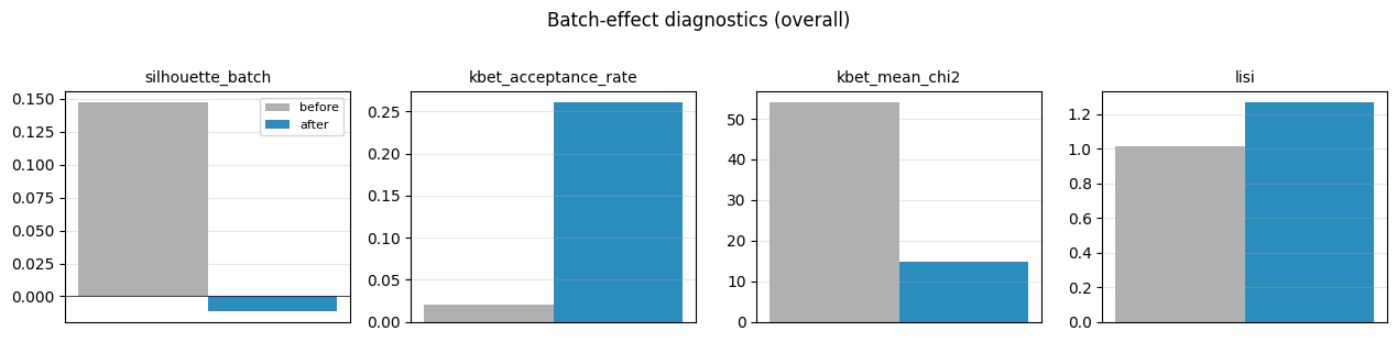
| 0 | silhouette_batch | overall | 0.147457 | -0.011313 | -0.158770 | lower |
| 1 | kbet_acceptance_rate | overall | 0.020243 | 0.260459 | 0.240216 | higher |
| 2 | kbet_mean_chi2 | overall | 54.016409 | 14.849020 | -39.167389 | lower |
| 3 | lisi | overall | 1.014542 | 1.265755 | 0.251213 | higher |
4. Plot the before / after summary#
[5]:
%matplotlib inline
from maldibatchkit.viz import plot_diagnostic_summary, plot_peak_shift
import matplotlib.pyplot as plt

fig, axes = plot_diagnostic_summary(report, scope='overall')
plt.show()
[6]:
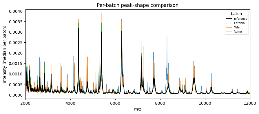
fig, ax = plot_peak_shift(ds.batch, ds.X, mz_values=ds.mz, max_batches=None)
ax.set_xlim(2000, 12000)
plt.show()
[7]:
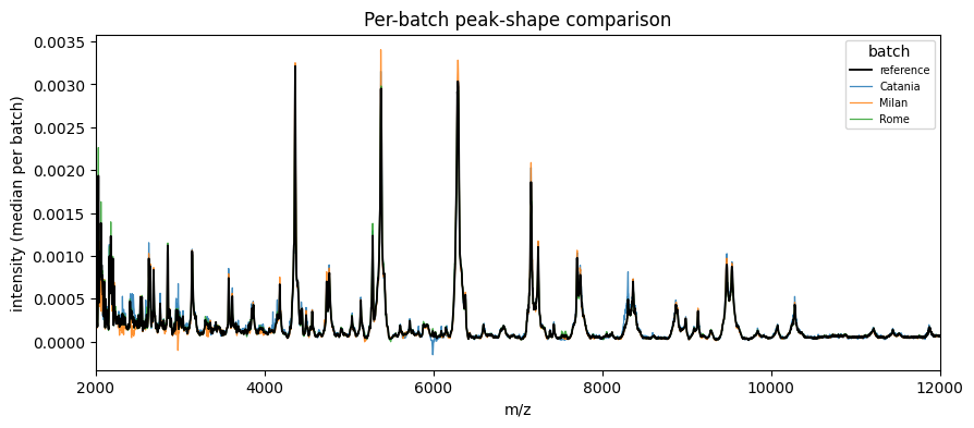
fig, ax = plot_peak_shift(ds.batch, X_corrected, mz_values=ds.mz, max_batches=None)
ax.set_xlim(2000, 12000)
plt.show()
Where next#
02_correction_methods.ipynb - side-by-side comparison of every corrector.
03_quality_weighted_combat.ipynb - deep dive into the quality-weighted empirical-Bayes extension.
04_maldiset_integration.ipynb - end-to-end workflow using
maldiamrkit.MaldiSet.